by A. Pomberger, N. Jose, D. Walz, J. Meissner, C. Holze, M. Kopczynski, P. Müller-Bischof, A.A. Lapkin
Abstract
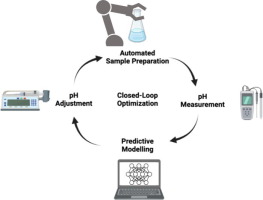
Buffer solutions have tremendous importance in biological systems and in formulated products. Whilst the pH response upon acid/base addition to a mixture containing a single buffer can be described by the Henderson-Hasselbalch equation, modelling the pH response for multi-buffered poly-protic systems after acid/base addition, a common task in all chemical laboratories and many industrial plants, is a challenge. Combining predictive modelling and experimental pH adjustment, we present an active machine learning (ML)-driven closed-loop optimization strategy for automating small scale batch pH adjustment relevant for complex samples (e.g., formulated products in the chemical industry). Several ML models were compared on a generated dataset of binary-buffered poly-protic systems and it was found that Gaussian processes (GP) served as the best performing models. Moreover, the implementation of transfer learning into the optimization protocol proved to be a successful strategy in making the process even more efficient. Finally, practical usability of the developed algorithm was demonstrated experimentally with a liquid handling robot where the pH of different buffered systems was adjusted, offering a versatile and efficient strategy for a pH adjustment processes.
Graphical Abstract
Introduction
Adjusting pH is an important step in the production of cosmetic formulations, liquid detergents, treatment of
industrial wastewater or within biopharmaceutical
drug manufacturing [1],
[2],
[3],
[4],
[5],
[6]. The process itself is often very time intensive due to complex proton partitioning equilibria and represents a challenging control problem resulting from the intrinsic non-linearity of the pH value
[7]. Additionally, buffer chemicals, weak acids or bases that can donate or accept protons, often used in the formulations to maintaining the pH within a narrow margin upon acid/base addition, complicate the process of pH adjustment. While single buffered systems can be described using the Henderson-Hasselbalch equation, developing models for multiple poly-protic buffers (e.g., phosphate and citrate) remains an ongoing challenge
[8],
[9].
Commercial and literature-reported pH adjustment strategies are typically either based on proportional-integral-derivate (PID) control or model
predictive control (MPC); both come with limitations. The PID control strategy continuously calculates deviation of the measured value from the target value, and applies a correction based on a proportional, integral or derivative correction strategy
[10],
[11]. A typical example are
bioreactors which often operate in fed-batch mode, relying on PID pH control to allow for the maintenance of specific conditions required by the biological cultures
[12],
[13],
[14],
[15]. While no chemical information except the continuous measured pH is needed for PID, a loss of information needs to be accepted since insights into the chemical system cannot be implemented into future pH adjustments, as opposed to model based strategies. More recent pH adjustment approaches are based on MPC arrays, e.g., Altinten
et al. describe a generalized predictive control for continuous flow pH adjustment
[16], Helmy
et al. relied on multi-linear regression
[17] and Alkamil
et al. used a fuzzy
artificial neural network (ANN) outperforming a PID-control
[18]. Others have also expanded on using ML based MPC strategies for this same purpose
[19],
[20]. A major challenge associated to MPC-based pH adjustment is operating in a low data regime, particularly of interest for high-throughput small-scale pH adjustment, as opposed to continuous pH adjustment. Aside from automated strategies, pH adjustment process is also often conducted manually in a R&D stage which is time consuming, requiring approximately-five to seven minutes per sample (
Table 1: entries 7, 10, 13).
The modern digitalization of research facilities allows the relatively fast and easy accumulation of experimental data, which can be used to accelerate subsequent workflows by employing
transfer learning (TL). TL represents the method of pretraining ML models for one task and subsequentially using the trained model for a similar prediction task
[21]. Typically, the
auxiliary model would profit from an availability of large pretraining datasets, whereas the target model is fine-tuned on a smaller dataset
[22],
[23],
[24],
[25]. Process chemists often modify the composition of formulated products (e.g., liquid laundry detergents) to fine tune product properties (e.g., viscosity). While small modifications do not change the overall composition greatly, the pH response (titration curve) does change and thus the sample requires a new titration strategy every time.
Herein, we aim to employ a data-driven strategy for pH adjustment, benefitting from active learning and robotic facilities for experimental evaluation. We compare different
surrogate models, machine-readable data representations and initialization strategies for the development of an active ML-based pH adjustment strategy of multi-buffered poly-protic mixtures. By employing TL, benefiting from previously generated data, we aim to demonstrate this novel strategy for pH adjustment and keep the process efficient, even under an extreme low data regime.
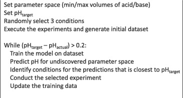
Our approach for active ML-driven closed loop optimization is shown in
Fig. 1a. A chosen ML model is initially trained within a low data regime (here three datapoints) and used for predicting the unknown (ground truth) full titration curve (
Fig. 1b). Subsequently, conditions towards the target pH are selected using a custom acquisition function. In active learning and
Bayesian optimization the acquisition function is typically a trade-off between exploration to reduce model uncertainty and exploitation towards the target value. For the pH adjustment we choose a purely exploitative approach by selecting the minimizer of the difference between the model predictions and the target pH as the next experimental condition (
Fig. 1c). This is possible as the pH curve is monotonous, hence the algorithm will converge to the target pH. Until the target pH has been reached, the dataset is continuously updated and the model is retrained for the next iteration. We coupled our active ML-guided pH adjustment approach with a liquid handling robot and successfully adjusted a set of chemically different binary buffered mixtures. After a comparison of different surrogate models, we identified Gaussian processes (GP) as the best performing model. Moreover, we managed to boost efficiency of the process by utilizing TL strategies, thus decreasing the required iterations of pH adjustment.
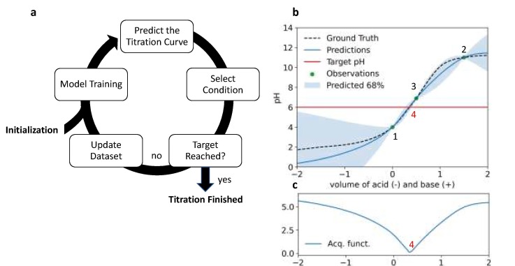
Fig. 1. An overview of the ML-driven pH adjustment strategy (a) Design of the closed-loop optimization toward pH adjustment (b) Illustration of ML model predictions and decision making using the acquisition function, see minimum at 4. (c). The numbers represent the order of the observations, and the red font color represents the datapoint to be acquired in the next iteration. Both acid and
base volume addition are represented on the x axis, where the negative values account for acid volume and the positive values account for base volumes.
Materials and methods
Active ML-driven closed-loop optimization
A chosen surrogate model is trained to map the input data (features) to the correlated output data (labels) – using a model-dependent data-processing architecture – by iteratively optimizing the model, i.e., minimizing the loss for all fitted datapoints
[26],
[27],
[28]. The predictive model performance is subsequentially evaluated on a held-out
test dataset – the model predictions are compared to the true values and the deviation is typically quantified via the residuals metric of
root mean squared error (RMSE). By applying this strategy in an iterative manner, it can be used to navigate through the parameter space, efficiently searching for desired conditions
[29],
[30],
[31]. In the case of pH adjustment this refers to the amount of acid or base to achieve a target pH. Algorithm 1 illustrates the control code used for automated pH adjustment.
To assess the performance of different surrogate models, particularly within a low data regime, and to deliver promising predictions, we conducted a comparative study between several models. Four commonly used ML models were chosen to understand their respective benefits and limitations: linear regression, random forest (RF)
[32], Gaussian process (GP)
[33] and artificial neural networks (ANN)
[34]. Hyperparameters for each model were optimized
a priori, see SI for more detail (Section 3). The initial approach intentionally did not implement chemical system information but solely generic one-hot encoding of the components and information on the addition of acid/base along with the respective system response. To understand whether the addition of chemical information such as component pKa values, number of protons a buffer can accept/donate and the initial pH value of the buffer mixture (prior to any acid/base addition) accelerates the process, a comparative study across all chemical systems was conducted, see comparison of small vs large feature set in
Fig. 4. The numerical values of the additional features were concatenated to the previous one-dimensional input vector.
Robotic platform
Based on the need to generate training data, as well as to demonstrate the active ML-based closed-loop pH adjustment process, we developed a robotic platform capable of mixing
buffer solutions, measuring pH value and automatically conducting pH adjustment (
Fig. 2). Here, the X/Y/Z labels refer to buffer
stock solution that can be pumped into glass vials (24 × 15 mL) positioned on the robotic wheel, acting as an auto sampler. On subsequent positions of the wheel, pH measurement and addition of acid/base can be conducted. After each pH adjustment process, the electrode is cleaned with deionized (DI) water to avoid cross-contamination between the samples. Technical design of the bespoke robotic platform was based on previous studies
[35],
[36]. We utilized FLab, a Python-based library, for facilitating communication between the motors, pumps, the
pH electrode and the implementation of the ML based optimization algorithm
[37]. See SI (
Fig. S1) for more detailed images and information on the robotic platform.
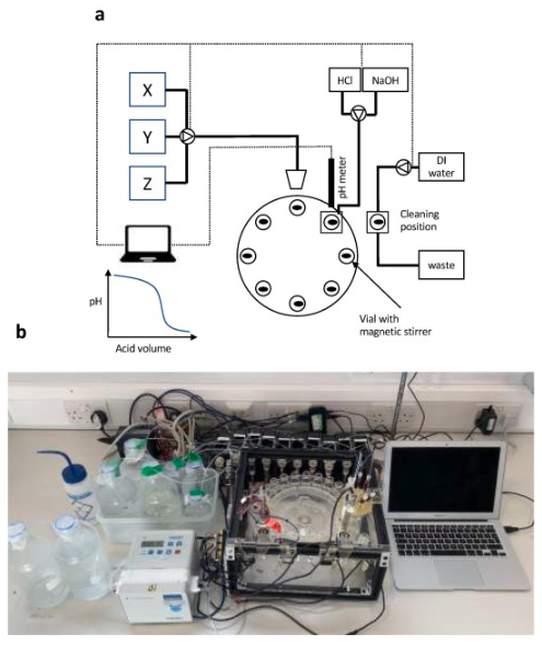
Fig. 2. Schematic (a) and image (b) of the robotic pH adjustment platform. X/Y/Z indicate the
stock solutions of buffer chemicals. For simplification not all 24 vials have been drawn on the robotic wheel. See SI for detailed labelled explanation of all components.
Results and discussion
Closed-loop optimization pH-adjustment
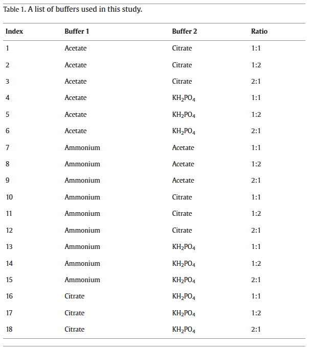
The performance of pH adjustment can vary significantly, depending on the complexity of the system response towards the addition of a titrating agent. To demonstrate the broad applicability of the pH adjustment strategy, we tested our approach on a variety of different chemical systems. 18 experimentally generated datasets of binary buffered mixtures, containing the acid/base volume addition as the input and the measured pH value as the output were used, see
Table 1. Based on the existence of this experimental data, simulated closed-loop optimization was conducted. The majority of the datapoints were held out and only a randomly selected batch of datapoints for initializing the model was used. The strategy (
Fig. 1) was applied, and the target pH was set to pH 6, with an acceptable deviation of a pH value of ± 0.2. For mixture 6 the initial pH of the sample was already within the target pH margin so the objective was set to pH 8. pH adjustment within this work was aimed to suit the requirements of cosmetic/agriculture formulations; it should be noted that biological buffer systems require a narrower gap within the adjustment step. This workflow was conducted 10 times for each dataset and the mean/standard deviation of the number of iterations needed to achieve the target pH were calculated.
Featurization included the concentration of both buffer chemicals, the volume of acid/base as well as chemical information such as pKa values, the number of protons per buffer and the initial pH value.
Fig. 3a illustrates the varying prediction performance of four chosen surrogate models, using four observations for training. By comparing the single surrogate model predictions against the ground truth, it becomes visible that linear regression delivered the worst fit, as expected, whereas GP delivered the best performance. Moreover, the characteristic piece-wise constant predictions, arising from the decision-tree based model architecture of the RF are visible, see Loh
[38].
Fig. 3b illustrates the
optimization trajectory of ANN (buffer system 2) towards the target pH 6, i.e. how the model conducts sampling of experimental datapoints to find the target pH 6. It is visible that the algorithm initially requires approximately-two iterations to explore the response and then starts to exploit towards the objective.
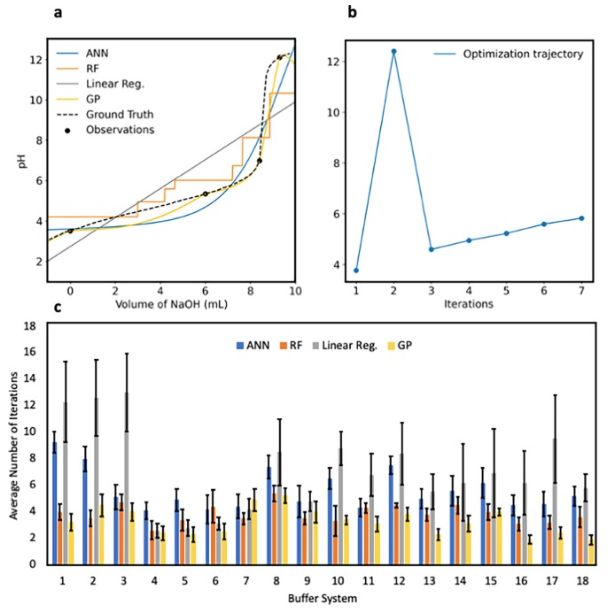
Fig. 3. Illustration of the active ML pH adjustment (a) Insights into prediction performance of four models after four observations (buffer system 1) and comparison to the ground truth. (b)
Optimization trajectory towards the target pH 6 (buffer system 2) using a
ANN surrogate model (c) Comparison of the required iterations to reach target pH using four different ML models for 18 different binary buffered systems. The features include the pKa values as well as the initial pH values. The error bars represent the error on mean value. See
Table 1 for indexed buffer system positions.
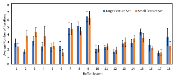
Fig. 4. Illustration of the required active learning iterations using GP to reach target pH for a set of buffer systems using two feature sets. Error bars represent the error on the mean value. See
Table 1 for information on the indexed buffer system positions.
A broad comparison of the 18 buffer systems and the choice of the ML model was conducted to assess the required number of iterations to conduct pH adjustment (
Fig. 3c). Chemical systems with multiple protons tend to have more linear areas whereas a system comprised of two single chemicals (e.g., ammonium, acetate) tends to be less smooth, see SI
Fig. S2. In addition to the number of protons, the pKa values are also important as they indicate the location of the
inflection point that will likely influence the system response of the
binary mixture. Systems containing two poly-protic buffers (e.g. citrate and phosphate) tend to require fewer iterations compared to systems containing monoprotic buffers such as ammonium or acetate. Given the variety of the tested buffer chemicals, we believe that a wide variety of buffer systems can be represented using the dataset, i.e. the strategy should be applicable to samples containing other pH-sensitive chemicals which are not directly represented in this study.
Linear regression clearly seems not to fit the datapoints well due to non-linear pH response, but it was conducted as a reference. It requires a high number of iterations for systems containing many polyprotic components, e.g., citrate, see
Fig. 3a,b. Overall, most of the systems could be adjusted within 3–4 iterations using three datapoints to initialize the optimization, thus giving a total of 6–7 required steps. On average, RF required 3.4 ± 0.3 iterations, ANN required 5.6 ± 1.0 iterations and GP required 3.1 ± 0.6. Here and in the following the reported values refer to the mean and the error of the mean value of 10 single iterations, see SI Eqn. S2. Our analysis shows that using the GP model gives the best results with the lowest number of iterations within the optimization loop.
Featurization effects
Representing chemical compounds in a machine-readable format is considered a challenge in chemoinformatics due to its effect on different surrogate models and, thus, their predictive performance
[39]. Previous literature has led to ambiguous outcomes on whether the addition of chemical information within low data regimes, such as the initialization of active-ML search strategies, is beneficial
[31],
[40]. To learn more about featurization effects on this specific application, we compared two input feature sets. The large feature set contains information on the components’ concentrations, component pKa values, number of protons a buffer can accept/donate and the initial pH value of the buffer mixture (prior to any acid/base addition). The small feature set contains only information on the components’ concentrations but no chemical insights.
As one can see in
Fig. 4, the performance of different informative features only minimally varies across the set of 18 systems. On average, using the large feature set resulted in 3.1 ± 0.6 iterations and the small feature set in 3.2 ± 0.6. While the results of the GP performance without chemical information might seem surprising, it must be noted that additional features increase the number of model parameters that need to be learned, as shown in other previously reported active ML studies by Pomberger
et al.
[40] Moreover, encoding pKa values of the components represents a challenge – depending on the used buffer 1–3 pKa values exist. To maintain fixed length of the input vector, the unused positions within the vector (e.g., ammonium only uses one spot whereas phosphate uses three spots) were filled up with zeros. We hypothesize that these steps might negatively influence the input format due to increased
sparsity. Moreover, the location of pKa values within the three slots for the numerical values might cause unwanted noise, e.g., the single pKa value for ammonium might be encoded as [9.25,0,0], [0,9.25,0] or [0,0,9.25].
The model initialization for each single system was conducted with 5 % of the training data instead of a consistent number of datapoints. While the number of initialization datapoints varies, the focus is on the relative comparison of the different feature sets.
As a result of the very similar outcome of the experiments (addition or exclusion of chemical information) it can be assumed that the strategy can be applied to chemical systems in a generic manner, specifically without exact knowledge of the chemical composition or
chemical structure – a challenge faced when e.g., working with confidential industrial data. Due to the slightly better performance, all further experiments were conducted using the large feature set within this study.
Variation of the number of datapoints for model initialization
The choice of the number of datapoints (obtained via random selection) for initializing the closed-loop cycle impacts the preliminary surrogate model’s prediction performance. While more initial datapoints could be considered as advantageous to train more accurate surrogate models, using fewer datapoints accelerates the overall adjustment process and might allow to selectively choose the subsequent datapoints based on the model’s prediction instead of initial random allocation. Within this case study we aim to identify this effect by comparing a GP, initialized with two, three and four random datapoints.
We investigated different sized initialization datasets for all 18 binary buffer systems, see
Fig. 5. When analyzing the results, we want to directly compare the total number of datapoints (i.e. pH measurements) required to obtain the target pH, hence the sum of the number of datapoints within the initialization dataset and the number of datapoints obtained during the experimental iterations. Overall, using only two initial datapoints resulted in the fastest method, requiring on average 5.8 ± 0.6 total pH measurements, followed by 6.3 ± 0.6 and 6.8 ± 0.5 pH measurements for three and four initial datapoints, respectively. When initializing a model with two datapoints, the subsequent two datapoints are chosen selectively as opposed to using four random datapoints for initialization. The results indicate that the selective choice of the active ML strategy seems to be beneficial over random datapoint allocation, irrespective of the fact that the preliminary model is solely trained on two datapoints.
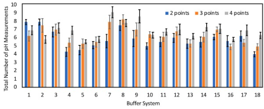
Fig. 5. Illustration of the effect of variation in the number of initialization datapoints on the total number of pH measurements necessary, using the large feature set and GP model. The deviation represents the calculated error on the mean value. See
Table 1 for information on the indexed buffer system positions.
Transfer learning-accelerated closed-loop optimization
Harvesting existing data to facilitate knowledge transfer was explored, to measure if preliminary models have a better understanding of the system response to acid/base additions, thereby accelerating the process of pH adjustment. In detail, we investigated whether prior knowledge of the pH response of single components may accelerate closed-loop pH adjustment of binary buffered mixtures. For example, information on pH response of ammonium and acetate was provided when conducting the pH adjustment of an ammonium-acetate sample. The titration information of the pure single-component buffer chemicals was combined with the initialization data and used for training the initial model. Both datasets were weighted equally during the learning process. As shown in
Fig. 6, the observable trend is that the addition of prior information improves the optimization performance.
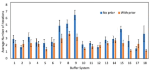
Fig. 6. Comparison of active ML-driven pH adjustment using GP and the full feature set with and without the implementation of prior information. The error bars represent the error on the mean value. Model initialization was conducted with 5% of the training data. See
Table 1 for information on the indexed buffer system positions.
Overall, using the GP alone without any prior information (just the initialization data) required 3.1 ± 0.6 iteration cycles, whereas, when implementing prior information of the single components, the number of iterations could be decreased down to 2.2 ± 0.4. Particularly challenging chemical systems, such as ammonium-acetate could be adjusted in significantly fewer number of iterations. While the results already suggest a strong increase in performance, we would like to note that further improvement might be possible via adjustment of the weighting parameter of prior data vs experimentally obtained data.
Real-time automated pH adjustment
After developing a strategy for automating the experimental workflow via a robotic platform along with an algorithmic strategy for controlling the addition of acid/base separately, we then aimed to merge both efforts. Using Flab, the control code of the liquid handling robot allows direct interaction with the algorithmic pH adjustment strategy – the measured data is directly used for ML surrogate model training. The results of the subsequent decision making (next conditions to evaluate experimentally) is passed to the liquid handling robot. The adjustment process and decision making can be monitored in real-time, as shown in
Fig. 1b.
While previous experiments were initiated with two – four randomly selected datapoints, we now initiated the pH adjustment process with a single datapoint aiming to decrease the overall number of required experimental observations. After initial pH measurement (volume of added acid/base = 0) the selected volume of titrant is added, and data acquisition commences.
Fig. 7 illustrates the results of the automated pH adjustment, representing the average of three single experimental evaluations. The plot indicates the clear differences between various buffered systems, ranging from two iterations (citrate–phosphate) to eight iterations (acetate-citrate). To demonstrate the performance of our approach for a chemically extremely complex equilibrium system and the feasibility of the GP to model the data we conducted successful pH adjustment of a sample containing up to four buffer chemicals. For a mixture of citrate, phosphate, ammonium and acetate the target pH 6 was achieved within 3.7 ± 0.4 iterations, thus demonstrating the versatility of the presented data-driven strategy. Overall, 4.7 ± 0.4 iterations were required to adjust the sample mixtures to the target pH 6.
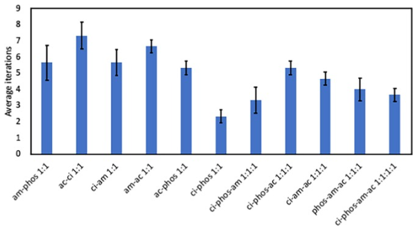
Fig. 7. Results of the experimental case study using the robotic platform and the developed active ML closed-loop algorithm to conduct automated pH adjustment of unknown buffered systems. For phos-am-ac 1:1:1 the target pH was set to 8 since the initial sample already yielded approximately a pH of 6. The error bars represent the error on the mean value, see SI Eqn. S2. Abbreviations: am: ammonium, phos: KH2PO4, ac: acetate, ci: citrate.
Conclusions
Within this study, we present a method to adjust the pH of several multi-buffered polyprotic solutions to aid
chemical laboratories dealing for formulation chemistry. A set target pH can be achieved via an iterative workflow in a fully automated manner, using a robotic platform informed by an active machine learning-based
optimization strategy.
Specifically, a Gaussian process was used to predict the titration curves of several mixtures and guide the pH adjustment towards a set target pH. Chemical inputs were featurized containing increasing levels of chemical information, delivering only marginally better efficiency. This can be regarded as advantageous since it allows to implement this approach for systems without the requirement of molecular information, particularly beneficial when dealing with confidential industrial formulation samples or when the composition of the sample has not yet been characterized in detail. Applying transfer learning to the optimization cycle significantly boosted the performance, thus highlighting the main advantage of ML-driven pH adjustment over PID controlled or manual pH adjustment. Since it is common for samples in high-throughput formulation preparation to differ in only one or a few parameters in their compositions, learning from previous pH adjustments and transferring the obtained system knowledge into a new pH adjustment process has been quantitatively shown to benefit the overall workflow.
In an attempt to balance the number of initially randomly chosen datapoints to selectively chosen datapoints it was observed that the overall sample efficiency improved when using less
initial data points. Finally, the strategy was demonstrated within a real experimental study with chemical systems containing up to four buffers – connecting the optimization algorithm and a robotic platform for conducting sample preparation and fully autonomous pH adjustment.
The developed workflow can be particularly beneficial for small scale high-throughput pH adjustment experiments as required by R&D facilities in formulation chemistry and may incentivize data accumulation and management for pH adjustment processes. Moreover, we see a great potential of this technique in the age of personalized cosmetics and medicine as well as all other small batch formulation processes.
Declaration of Competing Interest
The authors declare the following financial interests/personal relationships which may be considered as potential competing interests: Alexei Lapkin reports was provided by University of Cambridge.
Acknowledgments
A. Pomberger is grateful for funding of his PhD studies by BASF SE and EPSRC Centre for Doctoral Training “The Automated Chemical Synthesis Enabled by Digital Molecular Technologies” (SynTech CDT, EP/S024220). This work is co-funded by the EPSRC project “Combining Chemical Robotics and Statistical Methods to Discover Complex Functional Products“ (EP/R009902). We thank Dr Connor Taylor, Kobi Felton, Daniel Wigh and Ferdinand Kossmann for helpful discussions and providing feedback on the manuscript. We thank K. U. Thum for support with the experimental work. This work is co-funded by National Research Foundation (Singapore) grant “Cambridge Centre in Carbon Reduction Technologies”, via CREATE programme, and by European Regional Development Fund, via the project “Innovation Centre in Digital Molecular Technologies”.
Authors contributions
A. Pomberger developed the idea in discussions with D. Walz, J. Meissner, C. Holze and M. Kopczynski. A. Pomberger wrote the code and conducted the ML screening together with P. Müller. N. Jose developed and configurated the control code for the robot. AAL developed the project concept, secured funding and supervised the project. All authors discussed the results and contributed to the final manuscript.
Appendix A. Supplementary data
Data availability
Data will be made available on request.
References
-
J. Michl, K.C. Park, P. Swietach
Evidence-based guidelines for controlling pH in mammalian live-cell culture systems
Commun. Biol., 2 (1) (2019), p. 144
-
G.M. Alwan
pH-Control problems of wastewater treatment plants
Al-Khwarizmi Eng. J., 4 (2) (2008), pp. 37-45
-
R.K. Goel, J.R.V. Flora, J.P. Chen, Flow Equalization and Neutralization. In Physicochemical Treatment Processes. Handbook of Environmental Engineering, 2005; Vol. 3, pp 22-26.
-
M. Lukić, I. Pantelić, S.D. Savić
Towards optimal pH of the skin and topical formulations: from the current state of the art to tailored products
Cosmetics, 8 (3) (2021), p. 69
-
S. Hawkins, B.R. Dasgupta, K.P. Ananthapadmanabhan
Role of pH in skin cleansing
Int. J. Cosmet. Sci., 43 (4) (2021), pp. 474-483
-
T. Kalak, K. Gąsior, D. Wieczorek, R. Cierpiszewski
Improvement of washing properties of liquid laundry detergents by modification with N-hexadecyl-N, N-dimethyl-3-ammonio-1-propanesulfonate sulfobetaine
Text. Res. J., 91 (1–2) (2020), pp. 115-129
-
W.W. Tan, F. Lu, A.P. Loh, K.C. Tan
Modeling and control of a pilot pH plant using genetic algorithm
Eng. Appl. Artif. Intell., 18 (4) (2005), pp. 485-494
-
K.A. Hasselbalch
Die Berechnung der Wasserstoffzahl des Blutes aus der freien und gebundenen Kohlensaeuure desselben, und die Sauerstoffbindung des Blutes als Funktion der Wasserstoffzahl
Biochemische Zeit, 78 (1916), pp. 112-144
-
M.K. Nguyen, L. Kao, I. Kurtz
Calculation of the equilibrium pH in a multiple-buffered aqueous solution based on partitioning of proton buffering: a new predictive formula
Am. J. Physiol.-Renal Physiol., 296 (6) (2009), pp. F1521-F1529
-
S. Bennett
A brief history of automatic control
IEEE Control Syst. Mag., 16 (3) (1996), pp. 17-25
-
Y. Zhu, S. Nishigori, N. Shimura, T. Nara, E. Fujimori
Development of an automatic pH adjustment instrument for the preparation of analytical samples prior to solid phase extraction
Anal. Sci., 36 (5) (2020), pp. 621-626
-
U. Imtiaz, S.S. Jamuar, J.N. Sahu, P.B. Ganesan
Bioreactor profile control by a nonlinear auto regressive moving average neuro and two degree of freedom PID controllers
J. Process Control, 24 (11) (2014), pp. 1761-1777
-
S.W. Harcum, K.S. Elliott, B.A. Skelton, S.R. Klaubert, H. Dahodwala, K.H. Lee
PID controls: the forgotten bioprocess parameters
Discover Chemical Engineering, 2 (1) (2022), pp. 1-18
-
V. Chotteau, H. Hjalmarsson, In Tuning of Dissolved Oxygen and pH PID Control Parameters in Large Scale Bioreactor by Lag Control, Proceedings of the 21st Annual Meeting of the European Society for Animal Cell Technology (ESACT), , 2009; pp 327-330.
-
L. Hoshan, R. Jiang, J. Moroney, A. Bui, X. Zhang, T.-C. Hang, S. Xu
Effective bioreactor pH control using only sparging gases
Biotechnol. Prog., 35 (1) (2019), pp. 1-7
-
A. Altınten
Generalized predictive control applied to a pH neutralization process
Comput. Chem. Eng., 31 (10) (2007), pp. 1199-1204
-
H. Helmy, D.A.M. Janah, A. Nursyahid, M.N. Mara, T.A. Setyawan, A.S. Nugroho, In Nutrient Solution Acidity Control System on NFT-Based Hydroponic Plants Using Multiple Linear Regression Method, 2020 7th International Conference on Information Technology, Computer, and Electrical Engineering (ICITACEE), pp 272-276.
-
E.H.K. Alkamil, S. Al-Dabooni, A.K. Abbas, R. Flori, D.C. Wunsch
Learning From Experience: An Automatic pH Neutralization System Using Hybrid Fuzzy System and Neural Network
Procedia Comput. Sci., 140 (2018), pp. 206-215
-
N. He, M. Zhang, R. Li
An improved approach for robust MPC tuning based on machine learning
Mathematical Problems in Engineering, 2021 (2021), pp. 1-18
-
B.M. Åkesson, H.T. Toivonen, J.B. Waller, R.H. Nyström
Neural network approximation of a nonlinear model predictive controller applied to a pH neutralization process
Comput. Chem. Eng., 29 (2) (2005), pp. 323-335
-
S.J. Pan, Q. Yang
A Survey on Transfer Learning
IEEE Trans. Knowl. Data Eng., 22 (2010), pp. 1345-1359
-
G. Pesciullesi, P. Schwaller, T. Laino, J.-L. Reymond
Transfer learning enables the molecular transformer to predict regio- and stereoselective reactions on carbohydrates
Nat. Commun., 11 (1) (2020), pp. 1-8
-
Y. Zhang, L. Wang, X. Wang, C. Zhang, J. Ge, J. Tang, A. Su, H. Duan
Data augmentation and transfer learning strategies for reaction prediction in low chemical data regimes
Org. Chem. Front., 8 (7) (2021), pp. 1415-1423
-
Y. Amar, A.M. Schweidtmann, P. Deutsch, L. Cao, A. Lapkin
Machine learning and molecular descriptors enable rational solvent selection in asymmetric catalysis
Chem. Sci., 10 (27) (2019), pp. 6697-6706
-
C. Zhang, Y. Amar, L. Cao, A.A. Lapkin
Solvent selection for Mitsunobu reaction driven by an active learning surrogate model
Org. Process Res. Dev., 24 (12) (2020), pp. 2864-2873
-
M. Mohri, A. Rostamizadeh, A. Talwalkar, Foundations of machine learning. MIT press: 2012.
-
M.I. Jordan, T.M. Mitchell
Machine learning: Trends, perspectives, and prospects
Science, 349 (6245) (2015), pp. 255-260
-
G. Carleo, I. Cirac, K. Cranmer, L. Daudet, M. Schuld, N. Tishby, L. Vogt-Maranto, L. Zdeborová
Machine learning and the physical sciences
Rev. Mod. Phys., 91 (4) (2019), pp. 1-39
-
N.S. Eyke, W.H. Green, K.F. Jensen
Iterative experimental design based on active machine learning reduces the experimental burden associated with reaction screening
React. Chem. Eng., 5 (10) (2020), pp. 1963-1972
-
P. Jorayev, D. Russo, J.D. Tibbetts, A.M. Schweidtmann, P.P. Deutsch, S.D. Bull, A.A. Lapkin
Multi-objective Bayesian optimisation of a two-step synthesis of p-cymene from crude sulphate turpentine
Chem. Eng. Sci., 116938 (2021), pp. 1-10
-
B.J. Shields, J. Stevens, J. Li, M. Parasram, F. Damani, J.I.M. Alvarado, J.M. Janey, R.P. Adams, A.G. Doyle
Bayesian reaction optimization as a tool for chemical synthesis
Nature, 590 (7844) (2021), pp. 89-96
-
T.K. Ho, Random decision forests. Proceedings of 3rd International Conference on Document Analysis and Recognition 1995, 1, 278-282.
-
C.E. Rasmussen, C.K.I. Williams
Gaussian Processes for Machine Learning
MIT Press (2006)
-
J. Schmidhuber
Deep learning in neural networks: an overview
Neural Networks, 61 (2015), pp. 85-117
-
L. Cao, D. Russo, K. Felton, D. Salley, A. Sharma, G. Keenan, W. Mauer, H. Gao, L. Cronin, A.A. Lapkin, Optimization of Formulations Using Robotic Experiments Driven by Machine Learning DoE. Cell Reports Physical Science 2021, 2 (1), 100295 1-17.
- [36]
D.S. Salley, G.A. Keenan, D.-L. Long, N.L. Bell, L. Cronin
A Modular Programmable Inorganic Cluster Discovery Robot for the Discovery and Synthesis of Polyoxometalates
ACS Cent. Sci., 6 (9) (2020), pp. 1587-1593
-
Nicolas, J. FLab. https://pypi.org/project/flab/ (accessed 23.04.22).
-
W.-Y. Loh
Regression trees with unbiased variable selection and interaction detection
Statistica Sinica, 12 (2002), pp. 361-386
- D.S. Wigh, J.M. Goodman, A.A. Lapkin
A review of molecular representation in the age of machine learning
WIREs Comput. Mol. Sci., e1603 (2022), pp. 1-19
- A. Pomberger, A.A. Pedrina McCarthy, A. Khan, S. Sung, C.J. Taylor, M.J. Gaunt, L. Colwell, D. Walz, A.A. Lapkin
The effect of chemical representation on active machine learning towards closed-loop optimization
React. Chem. Eng., 7 (2022), pp. 1368-1379
This article is cited by
Science Direct