A Machine Learning-Enabled Autonomous Flow Chemistry Platform for Process Optimization of Multiple Reaction Metrics

Abstract

Self-optimization of chemical reactions using machine learning multi-objective algorithms has the potential to significantly shorten overall process development time, providing users with valuable information about economic and environmental factors. Using the Thompson Sampling Efficient Multi-Objective (TS-EMO) algorithm, the self-optimization flow chemistry system in this report demonstrates the ability to identify optimum reaction conditions and trade-offs (Pareto fronts) between conflicting optimization objectives, such as yield, cost, space-time yield, and E-factor, in a data efficient manner. Advantageously, the robust system consists of exclusively commercially available equipment and a user-friendly MATLAB graphical user interface, and was shown to autonomously run 131 experiments over 69 hours uninterrupted.

Graphical Abstract

A user-friendly MATLAB graphical user interface was utilized in combination with a robust machine learning self-optimization flow chemistry system to identify optimum reaction conditions and trade-offs (Pareto fronts) between optimization objectives, such as yield, cost, space-time yield, and E-factor, in a data efficient manner.

Introduction

Despite the prevalence of established techniques such as Design of Experiments (DoE), reaction optimization is still often a difficult and time-consuming task for chemists.¹ Identifying where improvements can be made is challenging due to the large number of process variables with many different possible combinations that should be tested. This issue can be alleviated using self-optimizing systems that combine programmable chemical handlers, a machine-learning reaction optimization algorithm, and online analytical techniques in a real-time adaptive feedback optimization loop (Figure 1). Examples of analytical methods suitable for self-optimising experimental systems include gas chromatography (GC), high-performance liquid chromatography (HPLC), mass spectrometry (MS), in-situ infrared spectroscopy (IR) and nuclear magnetic resonance (NMR) spectroscopy.² A significant advantage of these types of systems is that the optimization procedure can be entirely automated, where no user intervention is required.

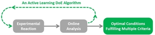
Figure 1
General flow chart of a reaction self-optimization system.

Reaction optimization conducted by chemists is typically measured against multiple performance criteria such as yield, cost, impurities profile, and environmental impacts. Therefore, the ability for the automated process to self-optimize for multiple objectives is highly desirable. The majority of existing self-optimizing systems utilize single-objective optimization algorithms, such as the Nelder-Mead simplex (NMSIM) and Stable Noisy Optimization by Branch and FIT (SNOBFIT).^3–5 Owing to the significantly increased complexity of multiple objective optimization, there are few algorithms that have been demonstrated to efficiently perform this task. Whilst multiple objectives can be scalarized into a single function, the weighting given to individual objectives is subjective when compared to multi-objective optimization.

Another key point for multi-objective algorithms is that objectives sometimes compete with one another (e. g. yield vs. cost), which makes it is impossible to find a single set of ‘utopian’ conditions that correspond with optimal values for both objectives. One representation of competing multi-objective optimization is a Pareto front (Figure 2),⁶ which is a set of non-dominated data points where either objective cannot be improved without having a detrimental effect on the other, i. e. showing the trade-off between objectives. An example of an algorithm for efficient multi-objective reaction optimization is the open-source Thompson Sampling Efficient Multi-Objective (TS-EMO).⁷ Lapkin and co-workers^6, 8–10 have demonstrated the quality of the generated Pareto fronts, as well as the algorithm’s efficiency at identifying them, when compared with alternative algorithms such as ParEGO.¹¹ Alternative examples multi-objective algorithms¹² developed for chemical process include Phoenics¹³ and Chimera.¹⁴

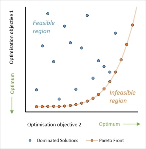
Figure 2
An illustration of a Pareto front (made up of non-dominated solutions) in a system with two competing optimization objectives, where values in the infeasible region under the Pareto front are inaccessible to the optimization process.

The application of flow chemistry over batch methods for self-optimizing systems has significant advantages. As well as being inherently safer under high temperature and pressure conditions (process intensification conditions), in situ analysis and closed-loop optimization systems are easier to implement in flow conditions as automated direct reaction sampling of the reaction solution can be performed using in-line small volume injectors or using non-invasive spectroscopic sampling. Furthermore, subsequent flow chemistry reactions can be conveniently initiated with different continuous reaction variables by modulating reactor temperatures and flow rates. Conversely, the screening of continuous variables in batch reactions is inefficient, typically requiring expensive robotic equipment.¹⁵

Self-optimization flow systems reported in the literature typically utilize custom-designed setups (consisting of pumps, reactors, samplers, and analytical equipment) interfaced with in-house software, which could be detrimental to the widespread adoption and rapid development of these tools. Furthermore, systems are sometimes developed for specific reactions, where modifying a system for a different reaction often requires considerable effort and time, even by experts.¹⁶ In contrast, the applications of commercially available modular flow chemistry systems, for example by Vapourtec, have been demonstrated to be effective in conducting many different reactions.^17–21 Furthermore, for more complex and scripted applications such as self-optimization, some systems can be remotely controlled through their standard software packages using application programming interfaces (API) written by manufacturers from popular programming environments in languages such as MATLAB or Python.

In this study we aim to further develop autonomous self-optimization flow chemistry systems, by developing a robust implementation, based on commercially available equipment and a proven ML algorithm, suitable for various single-step reaction optimization studies. The system has been demonstrated on a sample reaction exhibiting competing reaction pathways where optimisation of process parameters is known to lead to multiple possible “optimal” sets of reaction conditions. Here we also aim to further investigate the optimization behavior of the TS-EMO Bayesian optimizer with respect to exploitation vs exploration of experimental parameter space.

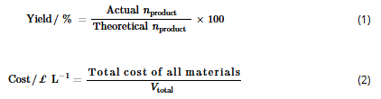
Results & Discussion

The case study reaction was the aldol condensation reaction between benzaldehyde (1) and acetone (2), catalyzed by sodium hydroxide (3) base, to give the desired benzylideneacetone (4) product (Scheme 1). The possible side-reactions to form dibenzylideneacetone (5) or acetone polymerization side-products represent an ideal challenge for careful control of reaction conditions chosen by the algorithm.

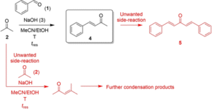
Scheme 1
Reaction scheme for the sodium hydroxide (3) catalyzed Aldol condensation case study between benzaldehyde (1) and acetone (2) to produce benzylideneacetone (4) at reactor temperature, T, with residence time, tres.

The self-optimization system utilized in this work features exclusively commercially available equipment and the TS-EMO multi-objective optimization algorithm (Figure 3). The flow chemistry equipment consists of two Vapourtec R2 modules and a R4 reactor module for controlling solution flows and reactor temperatures respectively. These parameters are controlled from within the software provided by the manufacturer.

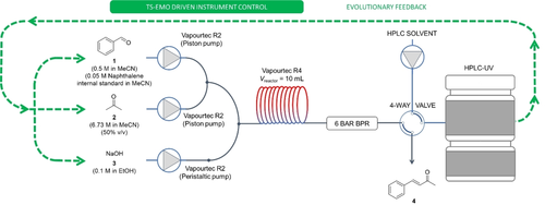
Figure 3
Schematic of the self-optimization systems containing a Vapourtec flow chemistry pumps and reactor, 4-way sample injector, HPLC-UV analysis, and algorithmic reaction optimization, controlled using a MATLAB based environment. BPR: back pressure regulator.

Designed for mesoscale flow chemistry,²² the system uses plug-flow modelling by calculating the flow rates and pump timings in relation to the desired reaction-zone plug sizes, determination of solution compositions within a plug, and automated signaling to reaction samplers and analytical equipment when the system is deemed to have reached steady-state. These features allow for easy implementation of direct reaction mixture sampling at steady-state using a microliter injector into an online HPLC-UV instrument. A bespoke MATLAB user interface was developed to control all aspects of the self-optimization process, including control of physical equipment through interface with commercial software, creation of training data sets, reading HPLC data and calculation of optimization objectives, and the complete, autonomous execution of flow chemistry experiments.²³ This process was repeated iteratively until the user terminated the MATLAB environment. It should be noted that any downstream processes, such as purification steps, were not taken into consideration in this work. Therefore, the cost and chemical use in these subsequent processes were not accounted for in the objective calculations.

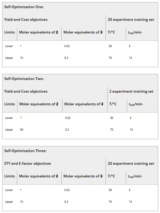
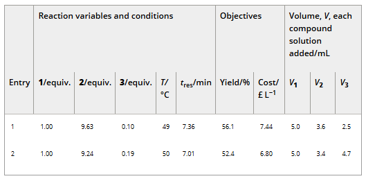
The four continuous variables optimized in all cases of this study were (i, ii) the molar equivalents of acetone and sodium hydroxide (relative to benzaldehyde), (iii) reactor temperature (T), and (iv) residence time (t_res), see Table 1 for user-defined lower and upper limits. Volume of benzaldehyde solution was fixed for each reaction. The upper limit for T was chosen as 70 °C to help avoid acetone polymerization, which results in poorly soluble products that clog the flow path and tubular reactor.²⁴ The residence time limits were set to ensure reactor pressure was not excessive with quicker experiments, whilst keeping total experiments to within 45 mins for longest experiments.

Table 1. Continuous variable limits for the self-optimisation of the aldol condensation reaction shown in Scheme 1. Molar equivalents is relative to the number of moles of 1. Solution concentrations: [1]=0.5 M in MeCN; [2]=6.73 M in MeCN; [3]=0.1 M in EtOH.

The first self-optimization performed in this study targeted reactions conditions that would maximize yield (Eq. 1) and minimize cost (Eq. 2). In Eq. 2, material costs were based on the prices at which they were purchased at the kg scale from a commercial supplier.

In Eq. 1, n_product is defined as the number of moles of product 4; in Eq. 2, the total cost of all materials refers to reaction solvents, reactants, and reagents, and V_total is the total volume of the reaction mixture. To initialize the TS-EMO algorithm, a training dataset of 20 experiments with values of the reaction conditions being optimized, was generated using Latin hypercube sampling (LHS) and autnomously performed. Figure 4).²⁵ Although previous studies have recommended 10 training experiments per continuous variable,²⁶ five experiments were selected in this instance based on the observed efficiency of TSEMO in previous experimental application.⁶

Figure 4
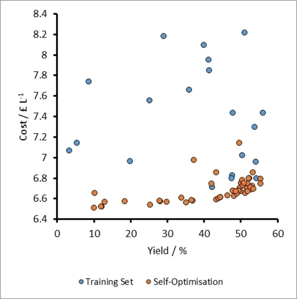
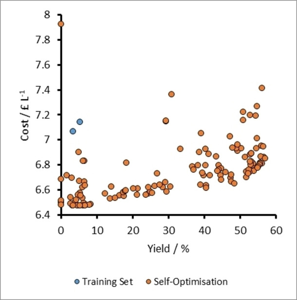
A plot of cost vs yield for experiments related to the self-optimization of aldol condensation reaction in Scheme 1 with limits from Table 1 (Self-Optimization One). The initial training set experiments and self-optimization experiments combine to form a Pareto front and the trade-off between the two optimization targets.

Further 47 iterations were designed by the ML algorithm and rapidly converged to form a clear Pareto front, where the highest yield was 56.1 % at a cost of 7.44 £ L⁻¹. The lowest cost reaction was at 6.51 £ L⁻¹ but had a much poorer yield of 10.1 %, illustrating the trade-off between these two objectives (Figure 4). The Pareto front shows how the yield can be significantly increased from 10.1 to 53.4 % for relatively minor increases in cost from 6.51 to 6.70 £ L⁻¹. The variable that had the greatest contribution to this significant increase in yield was the equivalents of relatively inexpensive acetone (Figure 5). The reasons for this are likely through mitigating the formation of side-product 5 and increasing the reaction rate to form the desired product 4 via increased concentration of 2. However, it is also clear that increasing the acetone equivalents has a small detrimental effect on the cost (Figure 5). A minor increase in yield from 53.4 to 56.1 % on the Pareto front corresponds to the large increase in the cost from 6.70 to 7.44 £ L⁻¹. When the reaction conditions for the costliest data point on the Pareto front (Table 2, Entry 1) is compared with two data points in the cluster just before the sharp increase in cost (Table 2, Entry 2), the main cause for the large cost difference was molar equivalents of sodium hydroxide used. The lower equivalents used for the costly experiment (0.10 equiv.) compared to the other data points (0.19 equiv.) resulted in approximately half the volume of sodium hydroxide solution being pumped into the reaction, which meant the benzaldehyde and acetone solutions accounted for a greater proportion of the total reaction volume. Therefore, the high calculated cost can be explained by the relatively high prices of benzaldehyde and acetone (see ESI for material prices).

Figure 5
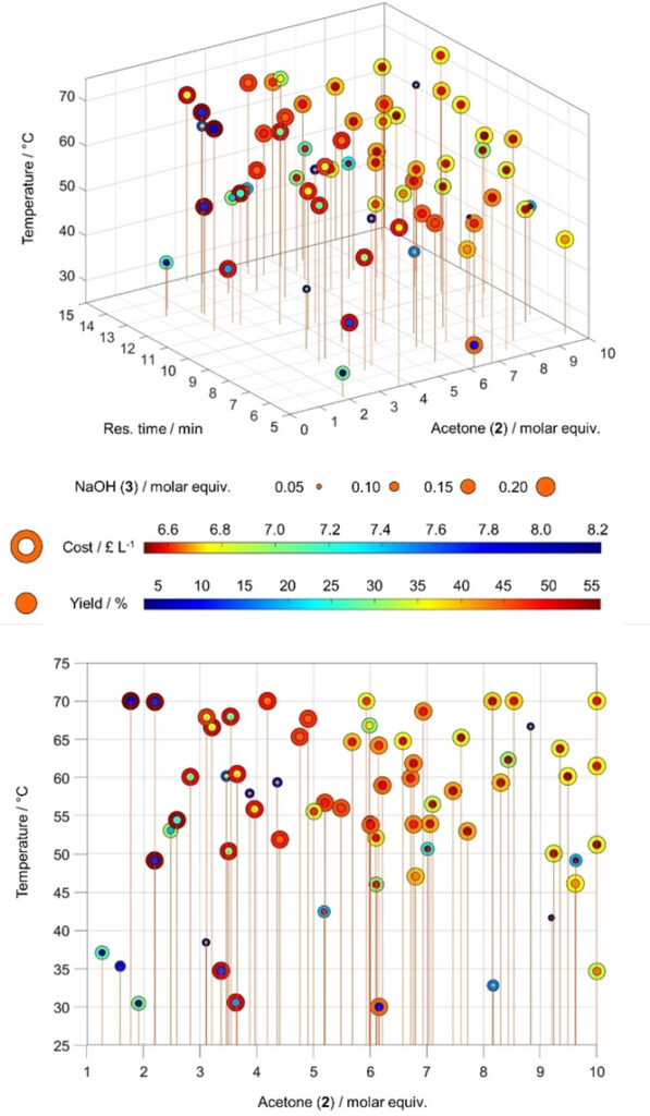
3D (upper) and 2D (lower) plots of experiments run in the Self-Optimization One of the aldol condensation reaction depicted in Scheme 1. Each point represents a single experiment executed during the optimization. The graph displays five variables as follows: (x) molar equivalents of 2, (y) residence time in the heated reactor (z) temperature of reactor. The point size denotes the molar equivalents of 3 in each run. The core color of each point represents the yield (%), whilst the shell color represents the cost of each experiment (£ L−1), as shown in the legend. Lower figure is identical to upper but rotated to depict data as viewed along the y-axis.

Table 2. Table of reaction variables and conditions, objective values, and volumes of each compound solution added (V_n where n=1, 2 or 3 corresponds to benzaldehyde, acetone and sodium hydroxide respectively) of two representative data points from the self-optimisation of the aldol condensation reaction shown in Scheme 1 with limits from Table 1 (Self-Optimization One), showing the difference in cost value as a result of solution volumes added.

In contrast to the effects of reactant/reagent molar equivalents on the target objectives, Figure 5 shows poor correlation between t_res and either yield or cost objectives. Whilst reaction temperature, T, was found to have no correlation with cost, it did exhibit positive correlation with yield. As shown in Figure 5, improvements in yield are observed when increasing temperature from 30 °C to above 50 °C.The reaction conditions used in the 67 experiments showed that the optimization algorithm often selected molar equivalents of acetone and sodium hydroxide close to the upper limit (a complete list reaction conditions for all experiments is available in the ESI). As mentioned previously, after 20 training experiments, the algorithm immediately converged to form the Pareto front. Therefore, with respect to the trade-off between exploration and exploitation of the optimization space typically observed in Bayesian optimization processes,^27, 28 the system described in this work demonstrated a greater tendency towards exploitation.This behavior is analogous to earlier chemical reaction optimizations using the TS-EMO algorithm reported by Bourne and Lapkin and co-workers.⁶ The relatively small number of training experiments required for the efficient optimization observed was proposed to be due to the wide range of experimental conditions, and yield and cost values in the initial training set data.²⁸To further investigate the exploration and exploitation characteristics of the TS-EMO algorithm and identify its effectiveness in locating the Pareto front, the optimization process was repeated but with only two poorly yielding experiments in the initial training set. In addition, the upper limit for the molar equivalents of acetone variable was increased to 50 equiv. to potentially allow for a greater variation in the yield and cost objectives (Table 1), since the previous optimization experiments were often conducted near the 10 eq. upper limit.Using two training experiments with yields of 3 % and 5 %, the system performed an additional 129 TS-EMO-designed experiments autonomously without interruption or error for 69 hours (full list of reaction conditions for all experiments is available in the ESI). After the initial six optimization iterations, the reaction conditions selected by the algorithm already generated yield and cost values close to the Pareto front, as shown in Figure 6. This further demonstrates the algorithm’s tendency to efficiently exploit, rather than explore the optimization space when locating the Pareto front. The increased scatter in the optimization experiments when compared with the initial optimization of 47 experiments, however, does indicate that algorithm retains a proclivity to explore when the uncertainty in relation to the pareto front is low. As the spread of reactions in the pareto region is far greater in this extended optimization when compared to the original run, it could be argued that an optimal number of training experiments helps to improve the efficiency of the optimization process.

Figure 6
A plot of cost vs yield for experiments related to the self-optimization of aldol condensation reaction in Scheme 1 with limits from Table 1 (Self-Optimization Two). The self-optimization experiments combine to form a Pareto front and the trade-off between the two optimisation targets.

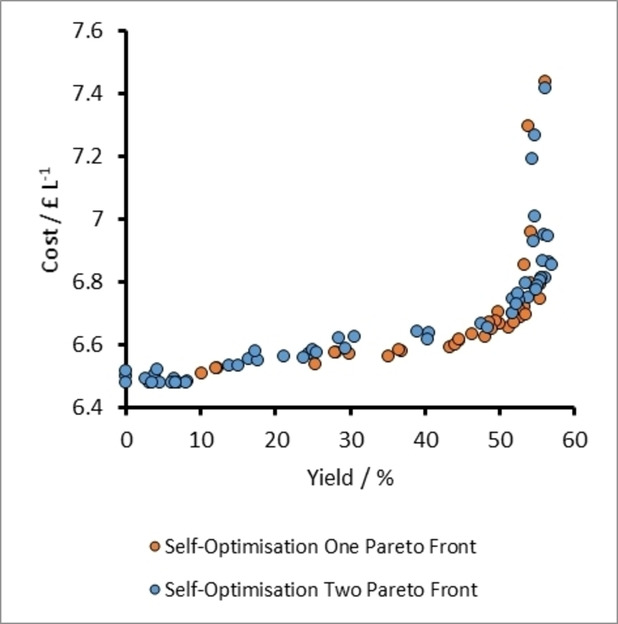
The cost vs. yield Pareto fronts produced from the two optimizations using different initial training sets are comparable (Figure 7), which suggests that acetone equivalents above 10 had a negligible effect on these objectives.

Figure 7
Plots for cost vs yield for specific experiments on the Pareto front related to the self-optimization of aldol condensation reaction in Scheme 1 with limits from Table 1.

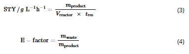
The final self-optimization performed in this study targeted reactions conditions that would maximize space-time yield (STY) and minimize the environmental impact using the E-factor metric. Space-time yield is a measure of reactor productivity related to the mass of product 4 formed (m_product), the reactor volume (V_reactor), and t_res (Eq. 3); whilst E-factor²⁹ is defined as the ratio of the mass of waste (m_waste) to m_product (Eq. 4.

The same initial training set of 20 experiments from the previous optimizations, as well as the same lower and upper variable limits (Table 1) were used to commence the process. It should be noted that a plot of log₁₀(E-factor) against STY, for the original training set was not spread across the optimization space as it had been for the previous optimizations (Figure 8). This suggested that there was no trade-off between the targets and therefore there could be a utopian optimum in this instance. The results after 55 TS-EMO optimization iterations confirmed that there was no Pareto front for these objectives, and instead identified an optimum where STY was 237.43 g L⁻¹ h⁻¹ and E-Factor=39.7 (Figure 8). Like the optimal conditions for the maximum yields in the previous optimizations, the ideal reaction conditions for achieving high STY and low E-factor corresponded to high acetone equivalents (9.94 equiv.), as well as a low t_res of 5.1 min. The absence of a Pareto front is due to the closeness of densities of benzaldehyde, acetone and sodium hydroxide solutions (0.795, 0.785 and 0.792 g mL⁻¹ respectively; see ESI for derivation). As the solvent accounts for most of the waste generated, the amount of waste generated between experiments is very similar. This leaves both STY and E-factor being mostly dependent on product quantity, and therefore allowed an optimum result to be identified.

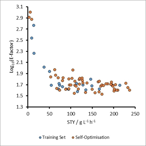
Figure 8
A plot of E-factor against STY for experiments related to the self-optimization of aldol condensation reaction in Scheme 1 with limits from Table 1 (Self-Optimization Three). In this case, there is an optimum solution for these two optimization targets, indicating there is no trade-off between them and therefore no Pareto front is present.

Conclusions

A self-optimization system consisting of a bespoke MATLAB user interface, a commercially available flow chemistry system, sampling and HPLC equipment and a self-optimizing algorithm was built and demonstrated autonomous uninterrupted operation for as many as 131 reactions over 69 hours. The multi-objective optimization algorithm was proven to be able to rapidly exploit the optimization space and locate optimum reaction conditions and key trade-off zones if competing objectives were under investigation. In the aldol condensation case study shown in Scheme 1, multi-objective optimizations to simultaneously maximize yield and minimize cost indicated that these two performance criteria competed with each other and formed a clear Pareto front. In contrast, optimizations to maximum STY and minimize E-factor converged towards a set of optimum reaction conditions.

Given the modularity of the commercial system employed, the flow chemistry setup can be easily modified with different supported components (such as pumps, tubing, reactors, purification modules) and/or additional chemical handlers for reactant loading/product collection. With respect to the handling of discrete variables, such as reagents and solvents, the TS-EMO optimizing algorithm was recently reported to be successful in optimizing for solvents in a ruthenium-catalyzed asymmetric hydrogenation reaction.¹⁰ Developments into handling discrete variables are currently underway in our laboratory, with the aim to demonstrate the improved capabilities and efficiencies using robotic workflows in process development.

Benzaldehyde was purified by washing with aqueous 10 % Na₂CO₃ solution, isolated by liquid−liquid separation, distilled under reduced pressure, and then stored under a nitrogen atmosphere. All other chemicals were used as received.HPLC analysis was performed using an Agilent 1260 Infinity system equipped with a G1311B quaternary pump, Eclipse XDB-C18 column (Agilent product number: 961967-302), and G1314F variable wavelength detector (VWD). Compounds were separated using the following HPLC quaternary pump method: the initial mobile phase was a 5 : 95 (v/v) binary mixture of acetonitrile and water flowing at 0.2 mL min⁻¹. Immediately after sample injection, the flow rate and ratio of acetonitrile and water were steadily changed to 1 mL min⁻¹ and 95 : 5 (v/v) during the first 5 min. At a flow rate of 1 mL min⁻¹, the binary mixture ratio is returned to 5 : 95 (v/v) acetonitrile:water over a duration of 1.5 min in a linear gradient. This binary mixture ratio is then held constant at 1 mL min⁻¹ for the next 1.5 min, after which the analysis is complete (after a total of 8 min), and the method returns to a flow rate of 0.2 mL min⁻¹. The VWD wavelength was changed over the 8 min analysis time as follows: the absorption wavelength was 254 nm for the initial 4.50 min, after it switched to 333 nm. After 1 min, the wavelength changed to 225 nm, then after an additional 0.57 min, the wavelength was returned to 254 nm.A schematic of the flow chemistry equipment and HPLC analysis components, as part of the self-optimization system are shown in Figure 3. Communication with the Flow Commander software for controlling the Vapourtec flow chemistry equipment was performed from a custom MATLAB user interface environment.²³ In this interface, the user selects the optimization variables and defines their limits, the physical properties of the reactants, HPLC parameters, the reaction scale, the optimization objectives, and the number of training experiments. Based on the flow rate of each reactant solution, Flow Commander calculated the time at which the reaction mixture is at steady state and automatically triggered the VICI Valco 4-port, 2 position sample injector to take a 60 nL sample from the flow path and send it to the HPLC system for analysis. Extraction of HPLC chromatogram retention times and peak areas, and calculation of yield, cost, STY, and/or E-factor occurred automatically after HPLC analysis was complete. The newly calculated values and all previous values were automatically inputted into the TS-EMO optimization algorithm, which in turn returned the reaction conditions for the next experiment in the optimization cycle (Figure 3). MATLAB then sent the new reaction conditions to Flow Commander for autonomous execution of the next reaction. In all experiments, the volume of benzaldehyde solution (with naphthalene as an internal standard), was kept constant at a user specified quantity. Throughout this study, a single experiment was executed, analyzed and processed by the ML algorithm before the conditions for the next experiment were generated. Complete tables of the reaction conditions used for all experiments can be found in the ESI.

Acknowledgements

The project is funded by Pharma Innovation Programme Singapore (PIPS).

Conflict of interest

The authors declare no conflict of interest.

References

Follow the link to the article below to click through to the references via the online article

This article is cited by

Chemistry Europe

References

[1] S. A. Weissman, N. G. Anderson, Org. Process Res. Dev. 2015, 19, 1605–1633.
[2] C. Mateos, M. J. Nieves-Remacha, J. A. Rincón, React. Chem. Eng. 2019, 4, 1536–1544.
[3] W. Huyer, A. Neumaier, ACM Trans. Math. Softw. 2008, 35, 1–25.
[4] M. W. Routh, P. A. Swartz, M. B. Denton, Anal. Chem. 1977, 49, 1422–1428.
[5] J. A. Nelder, R. Mead, Comput. J. 1965, 7, 308–313.
[6] A. M. Schweidtmann, A. D. Clayton, N. Holmes, E. Bradford, R. A. Bourne, A. A. Lapkin, Chem. Eng. J. 2018, 352, 277–282.
[7] E. Bradford, A. M. Schweidtmann, A. Lapkin, J. Glob. Optim. 2018, 71, 407–438.
[8] D. Helmdach, P. Yaseneva, P. K. Heer, A. M. Schweidtmann, A. A. Lapkin, ChemSusChem 2017, 10, 3632–3643.
[9] A. D. Clayton, A. M. Schweidtmann, G. Clemens, J. A. Manson, C. J. Taylor, C. G. Niño, T. W. Chamberlain, N. Kapur, A. J. Blacker, A. A. Lapkin, R. A. Bourne, Chem. Eng. J. 2019, 123340.
[10] Y. Amar, A. M. Schweidtmann, P. Deutsch, L. Cao, A. Lapkin, Chem. Sci. 2019, 10, 6697–6706.
[11] J. Knowles, IEEE Trans. Evol. Comput. 2006, 10, 50–66.
[12] C. A. Coello Coello, S. González Brambila, J. Figueroa Gamboa, M. G. Castillo Tapia, R. Hernández Gómez, Complex Intell. Syst. 2020, 6, 221–236.
[13] F. Häse, L. M. Roch, C. Kreisbeck, A. Aspuru-Guzik, ACS Cent. Sci. 2018, 4, 1134–1145.
[14] F. Häse, L. M. Roch, A. Aspuru-Guzik, Chem. Sci. 2018, 9, 7642–7655.
[15] M. B. Plutschack, B. Pieber, K. Gilmore, P. H. Seeberger, Chem. Rev. 2017, 117, 11796–11893.
[16] N. Cherkasov, Y. Bai, A. J. Expósito, E. V. Rebrov, React. Chem. Eng. 2018, 3, 769–780.
[17] P. R. D. Murray, D. L. Browne, J. C. Pastre, C. Butters, D. Guthrie, S. V. Ley, Org. Process Res. Dev. 2013, 17, 1192–1208.
[18] F. Lévesque, P. H. Seeberger, Angew. Chem. Int. Ed. 2012, 51, 1706–1709; Angew. Chem. 2012, 124, 1738–1741.
[19] B. Y. Park, M. T. Pirnot, S. L. Buchwald, J. Org. Chem. 2020, 85, 3234– 3244.
[20] E. T. Sletten, M. Nuño, D. Guthrie, P. H. Seeberger, Chem. Commun. 2019, 55, 14598–14601.
[21] M. Elsherbini, B. Winterson, H. Alharbi, A. A. Folgueiras-Amador, C. Génot, T. Wirth, Angew. Chem. Int. Ed. 2019, 58, 9811–9815.
[22] R. C. Wheeler, O. Benali, M. Deal, E. Farrant, S. J. F. MacDonald, B. H. Warrington, Org. Process Res. Dev. 2007, 11, 704–710.
[23] The MATLAB user interface and self-optimisation code (excluding proprietary Vapourtec code lines) is freely available on GitHub at http://github.com/cares-pips/mat-optimiser, 2020.
[24] M. I. Jeraal, N. Holmes, G. R. Akien, R. A. Bourne, Tetrahedron 2018, 74, 3158–3164.
[25] V. R. Joseph, Y. Hung, Stat. Sin. 2008, 18, 171–186.
[26] J. L. Loeppky, J. Sacks, W. J. Welch, Technometrics 2009, 51, 366–376.
[27] B. Shahriari, K. Swersky, Z. Wang, R. P. Adams, N. De Freitas, Proc. IEEE 2016, 104, 148–175.
[28] S. Sano, T. Kadowaki, K. Tsuda, S. Kimura, J. Pharm. Innov. 2019, 1–11.
[29] R. A. Sheldon, ACS Sustainable Chem. Eng. 2018, 6, 32–48.
Manuscript received: August 18, 2020
Version of record online: December 16, 2020